Intuitions
Better intuitions for algorithms — two-pointer elimination proofs, graph traversal mechanics, streaming median derivation, merge sort vs insertion sort information theory.
Two-Pointer Technique (Two Sum on Sorted Array)
About
The two-pointer technique uses two indices traversing a data structure in coordinated ways to solve problems efficiently (often O(n) instead of O(n²)).
Common applications:
- Two Sum on sorted array - Pointers at start/end, move inward based on sum
- Merge operation - Compare elements from two sorted arrays
- Palindrome check - Compare from both ends toward middle
- Sliding window - Define expanding/contracting ranges
- Partitioning - Swap elements around a pivot
- Cycle detection - Slow/fast pointers in linked lists
Better Intuition (close to a proof)
TL;DR: It’s an elimination argument, not a search. Each step safely eliminates one element that cannot possibly be part of any solution.
For Two Sum on a sorted array, explanations say “if sum is too large, move right pointer left” without explaining why this is safe.
Think of it as eliminating candidate elements that cannot possibly be part of the solution.
Given sorted array [a₀, a₁, ..., aₙ] and target sum T:
- Start with
s₀ = min + max(smallest + largest) - If s₀ > T: The sum is too large. But
maxis already paired with the smallest possible element. Somaxcannot be part of any valid pair — safely eliminate it from the candidates. - If s₀ < T: The sum is too small. But
minis already paired with the largest possible element. Somincannot be part of any valid pair — safely eliminate it from the candidates.
After safely eliminating one candidate, check s₁ on the remaining array. Repeat.
Note: we’re walking the space of sums in an interesting way — neither from smallest to largest nor largest to smallest, but along a path informed by the min/max elimination.
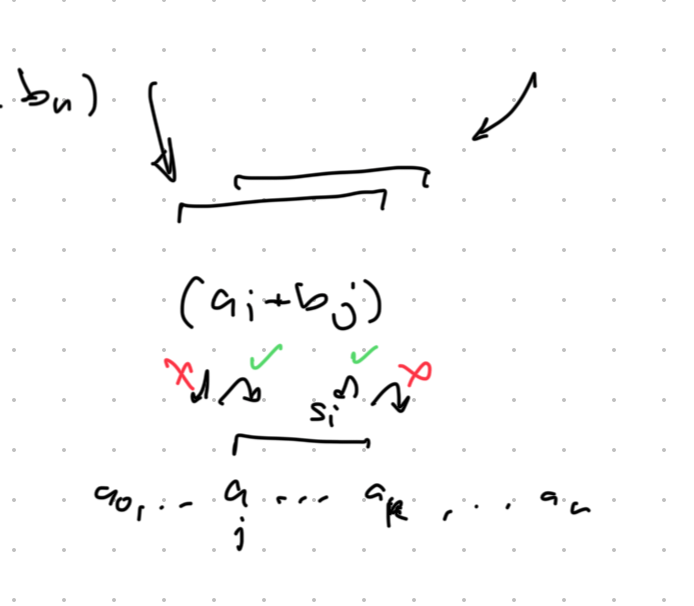
The image shows why the typical framing is counterintuitive: if you think of being at some sᵢ and comparing to the target, you have 4 choices (increment or decrement either pointer). But from the elimination view, there’s only one safe move — eliminate the candidate that cannot possibly work.
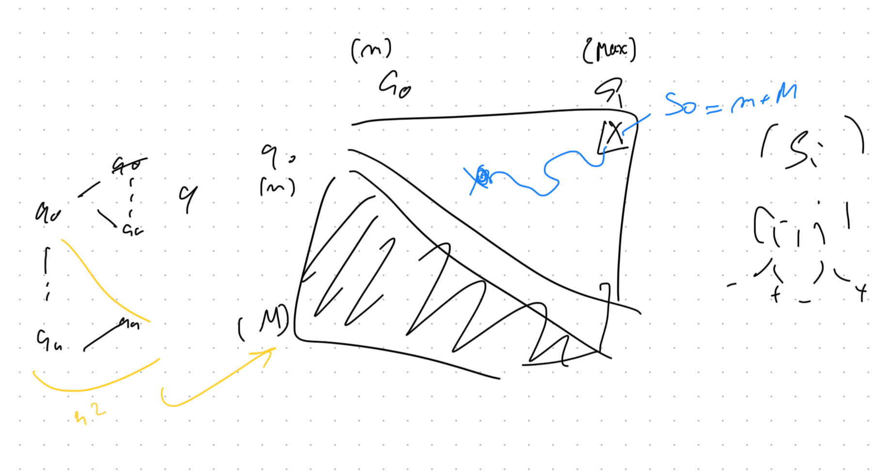
Tree/Graph Traversal, Recursion, Data Strucutues, Traversal Order
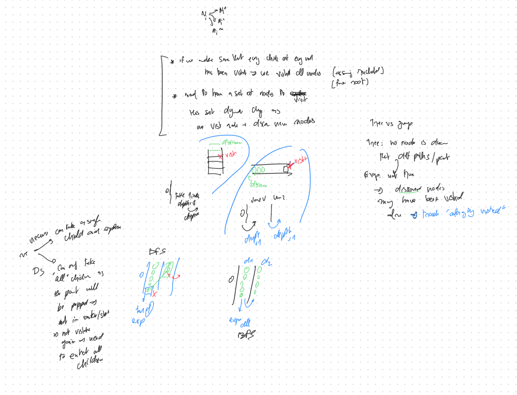
A tree is a graph. For traversal, what makes a graph more complex is that nodes can be reached from multiple parents (including forming loops). This is why we must track which nodes were visited, while in a tree, a node will natrually be visited once.
Core: Two Node States
Every traversal algorithm is about managing two sets:
| State | Meaning | Where it lives |
|---|---|---|
| Discovered | “I know you exist, you’re on my list” | Frontier (stack/queue/call stack) |
| Visited | “I’ve processed you and your neighbors” | Visited set (explicit or implicit) |
The traversal is just a loop:
1
2
3
4
while frontier is not empty:
    take node from frontier
    mark as visited
    discover its unvisited neighbors → add to frontier
That’s all. DFS, BFS, Dijkstra, A* — all variations on this theme.
What data structure holds discovered nodes?
| Structure | Retrieval Order | Algorithm | Gives You |
|---|---|---|---|
| Stack | Last discovered, first out | DFS | Deep paths first |
| Queue | First discovered, first out | BFS | Level-by-level, shortest path |
| Priority Queue | Lowest cost first | Dijkstra/A* | Optimal path by weight |
Recursion or explicit data structure?
| Approach | Pros | Cons |
|---|---|---|
| Recursion | Elegant, flexible, parent stays “live” | Stack depth limits, harder to pause/resume |
| Explicit Stack | No stack overflow, full control | More verbose, must capture all children eagerly |
| Queue | Required for BFS | Can’t use recursion naturally |
Recursion feels more natural for tree problems — you don’t need to eagerly capture everything before moving on
- DS: Once you pop a node, it’s gone. You must record all children into the frontier immediately, or you lose access to them forever.
- Recursion: The parent stays on the call stack while you explore. You have full flexibility — process children one at a time, in any order, with the parent context always available.
The State Transition Diagram
1
2
3
4
5
6
7
8
9
10
11
12
13
14
15
16
17
18
19
                    ┌─────────────┐
                    │  UNKNOWN    │
                    │ (not seen)  │
                    └──────┬──────┘
                           │ neighbor of visited node
                           ▼
                   ┌──────────────┐
        ┌──────────│ DISCOVERED   │◄────────┐
        │          │ (in frontier)│         │
        │          └──────┬───────┘         │
        │                 │ popped from     │
        │                 │ frontier        │
        │                 ▼                 │
        │          ┌─────────────┐          │
        │          │  VISITED    │──────────┘
        │          │ (processed) │ discovers neighbors
        │          └─────────────┘
        │
        └── In graphs: check before adding.
Deriving the Two-Heap Streaming Median
When we start with a couple of elements, it seems easy, let’s follow that, and try to hang on to the simple setup that we have, let’s try to “Hang on to the middle” — at every step, we need the median available.
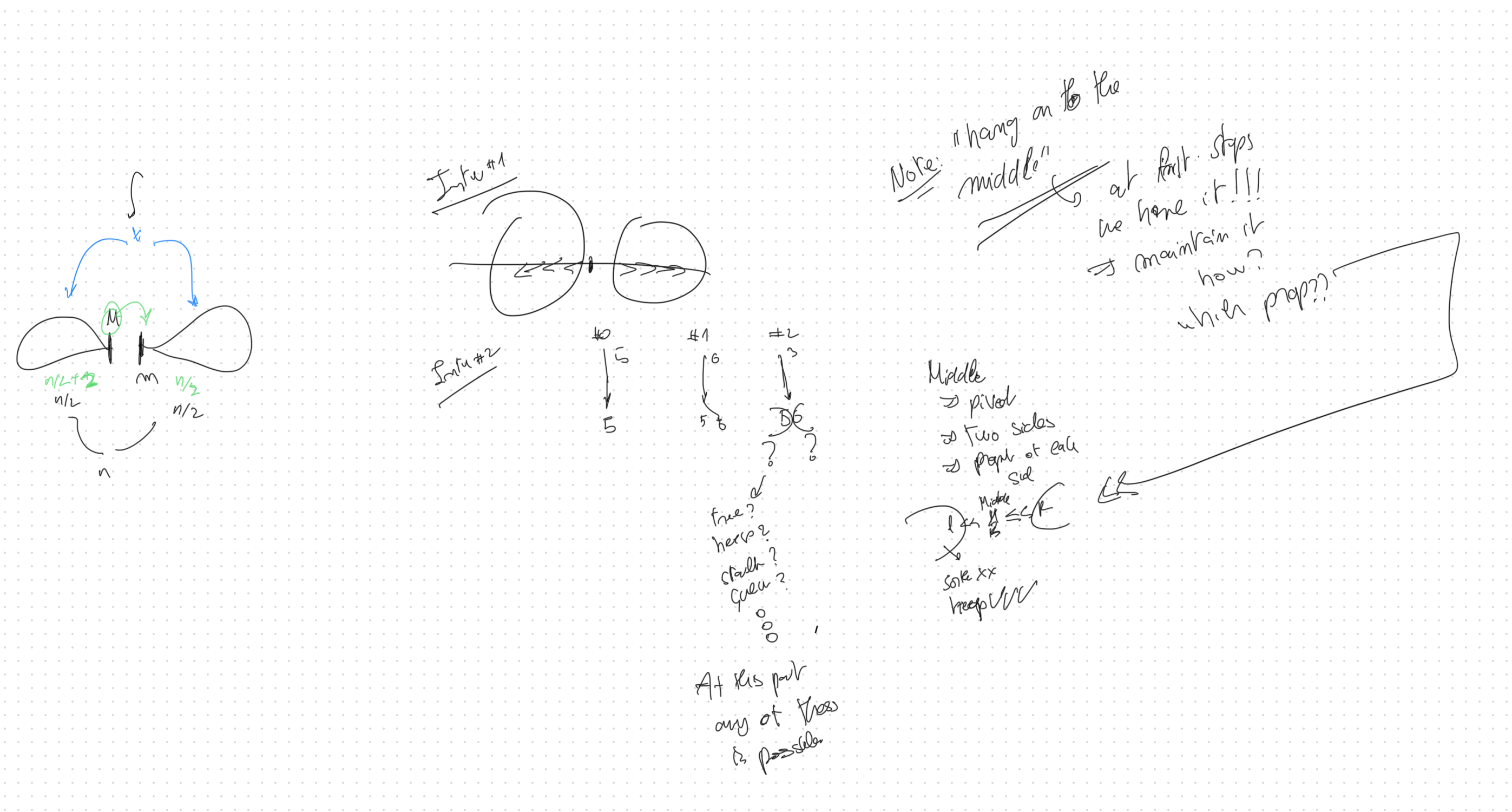
Start From Initial Conditions
We have 2 elements, adding a 3rd. Now we have:
- A middle element
- A left side (one element)
- A right side (one element)
The Subtle Moment
Stop here. Be subtle enough to notice: each side has exactly one element right now. Maybe, the element is part of some data structure that would allow us to maintain what we are hanging on to. At this point, the DS could be an array, maybe sorted, a graph, a tree, a heap…
Let’s ask: as more elements arrive, what property will each side need to maintain?
The left side: a collection where all elements are less than middle (<<<<) The right side: a collection where all elements are greater than middle (>>>>)
| Structure | Property | Fits? |
|---|---|---|
| Array | No ordering guarantee | ✗ |
| Sorted array | Full ordering (overkill, O(n) insert) | ✗ |
| BST | Left < root < right, but structure is scattered | ✗ |
| Map | Key-value lookup, not about ordering | ✗ |
| Heap | All descendants < root (max) or > root (min) | ✓ |
The heap property is exactly the “all less than” / “all greater than” property we need!
- Left side (
<<<<toward middle) → max-heap (root is largest = closest to middle) - Right side (
>>>>away from middle) → min-heap (root is smallest = closest to middle)
1
2
3
4
5
6
7
    MAX-HEAP          MIDDLE          MIN-HEAP

       [5]              7               [9]
      /   \                            /   \
    [3]   [4]                       [12]  [15]

    <<<<<<<            M              >>>>>>>
The median lives at the boundary: top of one heap, or average of both tops.
This seems to work out
We need to keep the two sides balanced (equal size, or off by one). This means sometimes moving elements across the middle.
We seem to be lucky: rebalancing preserves the properties we need.
- Pop from max-heap → gives us the largest of the left side (the one closest to middle)
- Push to min-heap → it’s smaller than everything already there ✓
The Mental Obstacle to Queue-Based Traversal
The core difficulty in using a Queue for Breadth-First Search (BFS) is the contrast between the Call Stack’s safety netand the Queue’s explicit amnesiaS).
Recursion Feels Natural
Recursion for tree traversal feels intuitive because the control structure is isomorphic (has the same shape) as the data structure.
- State Storage: When a recursive call is made, the operating system pauses the parent function’s state and pushes it onto the Call Stack. The stack grows as you descend the tree and shrinks as you return.
- Ancestry is Preserved: The history (ancestry) is preserved because the parent’s function call is simply paused. The stack mirrors the tree structure.
Queue: The Obstacle of Amnesia
The Queue mechanism of traversal is destructive and stateless regarding ancestry.
- Amnesic Operation: When you process a node you call
popleft()(dequeue). The Queue only holds the immediate frontier of nodes to visit next. - The Worry is True: The intuition—that the Queue cannot hold the state (ancestry)—is correct. The Queue is a destructive tool for discovery.
- Auxiliary Vector: Any problem requiring a structured result (like Level Order Traversal) needs an auxiliary data structure. One must manually archive the popped nodes (or values) into this external memory.
The Queue handles Traversal Order; the external Vector handles Context Preservation.
SHA Hardware Acceleration Instruction Cheat Sheat
SHA Hardware Acceleration Instructions
1
2
3
4
5
6
7
8
9
10
11
12
13
14
15
16
17
18
19
20
21
22
23
24
25
26
27
28
29
30
31
32
33
34
35
36
37
38
39
40
41
42
43
44
45
46
47
48
49
50
51
52
53
54
55
56
57
58
59
60
61
62
63
64
65
66
67
68
69
70
71
72
73
74
75
76
77
78
79
80
81
82
83
84
85
86
87
88
89
90
91
92
93
94
95
96
97
98
99
100
101
102
103
104
105
106
107
108
109
110
111
112
113
114
115
116
117
118
119
120
121
122
123
124
125
126
127
128
129
130
131
132
133
134
135
136
137
138
139
140
141
142
143
144
145
146
147
148
149
150
151
152
153
154
155
156
157
158
159
160
161
162
163
================================================================================
                    SHA HARDWARE ACCELERATION INSTRUCTIONS
================================================================================

ARM (ARMv8 Crypto Extensions)
─────────────────────────────────────────────────────────────────────────────────
Instruction     Data Width    Purpose                          Rounds/Words
─────────────────────────────────────────────────────────────────────────────────
sha256su0       128-bit       Message schedule σ0 + W[i-16]    4 words
sha256su1       128-bit       Message schedule σ1 + W[i-7]     4 words
sha256h         128-bit       Compression (first half)         4 rounds
sha256h2        128-bit       Compression (second half)        4 rounds

sha512su0       128-bit       Message schedule σ0 + W[i-16]    2 words
sha512su1       128-bit       Message schedule σ1 + W[i-7]     2 words
sha512h         128-bit       Compression (first half)         2 rounds
sha512h2        128-bit       Compression (second half)        2 rounds

sha1c           128-bit       SHA-1 rounds (choice)            4 rounds
sha1p           128-bit       SHA-1 rounds (parity)            4 rounds
sha1m           128-bit       SHA-1 rounds (majority)          4 rounds
sha1su0         128-bit       SHA-1 schedule part 1            4 words
sha1su1         128-bit       SHA-1 schedule part 2            4 words
sha1h           32-bit        SHA-1 fixed rotate               1 word
─────────────────────────────────────────────────────────────────────────────────
Introduced: ARMv8-A 2011 (SHA-1/256), ARMv8.2-A 2016 (SHA-512)


x86 Intel SHA-NI
─────────────────────────────────────────────────────────────────────────────────
Instruction     Data Width    Purpose                          Rounds/Words
─────────────────────────────────────────────────────────────────────────────────
sha256rnds2     128-bit       Compression rounds               2 rounds
sha256msg1      128-bit       Message schedule (σ0 part)       4 words
sha256msg2      128-bit       Message schedule (σ1 part)       4 words

sha1rnds4       128-bit       SHA-1 compression rounds         4 rounds
sha1nexte       128-bit       SHA-1 e accumulate + rotate      -
sha1msg1        128-bit       SHA-1 schedule part 1            4 words
sha1msg2        128-bit       SHA-1 schedule part 2            4 words
─────────────────────────────────────────────────────────────────────────────────
Introduced: Intel Goldmont 2016, AMD Zen 2017


x86 Intel SHA-512 Extensions
─────────────────────────────────────────────────────────────────────────────────
Instruction     Data Width    Purpose                          Rounds/Words
─────────────────────────────────────────────────────────────────────────────────
VSHA512MSG1     256-bit YMM   Message schedule (σ0 part)       2 words
VSHA512MSG2     256-bit YMM   Message schedule (σ1 part)       2 words
VSHA512RNDS2    256-bit YMM   Compression rounds               2 rounds
─────────────────────────────────────────────────────────────────────────────────
Introduced: Intel Arrow Lake / Lunar Lake 2024 — EVEX encoded
Detection: CPUID (EAX=07H, ECX=1) → EAX bit 0


x86 AVX Variants (V-prefixed)
─────────────────────────────────────────────────────────────────────────────────
Instruction     Data Width    Purpose                          Rounds/Words
─────────────────────────────────────────────────────────────────────────────────
VSHA256RNDS2    128-bit XMM   Compression rounds               2 rounds
VSHA256MSG1     128-bit XMM   Message schedule (σ0 part)       4 words
VSHA256MSG2     128-bit XMM   Message schedule (σ1 part)       4 words
─────────────────────────────────────────────────────────────────────────────────
Introduced: alongside SHA-512 extensions 2024


================================================================================
                         PROCESSOR SUPPORT MATRIX
================================================================================

Vendor              Year    SHA-1/256    SHA-512
─────────────────────────────────────────────────────────────────────────────────
Intel Goldmont      2016       ✅           ❌         Atom low-power
Intel Ice Lake      2019       ✅           ❌         Mobile
Intel Rocket Lake   2021       ✅           ❌         Desktop
Intel Alder Lake    2021       ✅           ❌         Desktop/Mobile
Intel Raptor Lake   2022       ✅           ❌         Desktop/Mobile
Intel Arrow Lake    2024       ✅           ✅         Desktop (Core Ultra 200S)
Intel Lunar Lake    2024       ✅           ✅         Mobile (Core Ultra 200V)
─────────────────────────────────────────────────────────────────────────────────
AMD Zen 1           2017       ✅           ❌         Ryzen 1000
AMD Zen 2           2019       ✅           ❌         Ryzen 3000
AMD Zen 3           2020       ✅           ❌         Ryzen 5000
AMD Zen 4           2022       ✅           ❌         Ryzen 7000
AMD Zen 5           2024       ✅           ❌         Ryzen 9000
─────────────────────────────────────────────────────────────────────────────────
ARM Cortex-A53+     2012       ✅           ❌         ARMv8-A
ARM Cortex-A75+     2016       ✅           ✅         ARMv8.2-A
Apple M1            2020       ✅           ✅
Apple M2            2022       ✅           ✅
Apple M3            2023       ✅           ✅
Apple M4            2024       ✅           ✅
─────────────────────────────────────────────────────────────────────────────────


================================================================================
                         THROUGHPUT COMPARISON
================================================================================

Algorithm    Scalar Ops/Block    HW Instructions    Theoretical Speedup
─────────────────────────────────────────────────────────────────────────────────
SHA-1             ~1200              ~40                  ~30x
SHA-256           ~2000              ~56                  ~35x
SHA-512           ~2500              ~36                  ~70x
─────────────────────────────────────────────────────────────────────────────────

Real-world throughput (approximate):
─────────────────────────────────────────────────────────────────────────────────
                        SHA-256              SHA-512
─────────────────────────────────────────────────────────────────────────────────
Software (scalar)       ~500 MB/s            ~300-500 MB/s
x86 SHA-NI              ~2-3 GB/s            N/A (software only)
x86 SHA-512 ext         ~2-3 GB/s            ~2+ GB/s
ARM + crypto ext        ~2-3 GB/s            ~3-5 GB/s
─────────────────────────────────────────────────────────────────────────────────

================================================================================
                                 GAPS
================================================================================

┌─────────────────────────────────────────────────────────────────────────────┐
│ 1. AMD SHA-512                                                              │
│    No hardware support across all Zen architectures (Zen 1-5, 2017-2024)    │
│    Must use AVX2/AVX-512 SIMD software implementations                      │
│    ARM has ~3-5x throughput advantage                                       │
├─────────────────────────────────────────────────────────────────────────────┤
│ 2. Intel SHA-512 (different older than 2024)                                      │
│    Arrow Lake and Lunar Lake only (2024)                                    │
│    Alder Lake, Raptor Lake, all Xeons: software only                        │
├─────────────────────────────────────────────────────────────────────────────┤
│ 3. x86 SHA-256 Compression Granularity                                      │
│    sha256rnds2 does 2 rounds (ARM sha256h/h2 does 4)                        │
│    x86 needs 2x more instructions for same work                             │
│    Partially offset by higher x86 clock speeds                              │
├─────────────────────────────────────────────────────────────────────────────┤
│ 4. SHA-3 / Keccak (all platforms)                                           │
│    No dedicated instructions on ARM, Intel, or AMD                          │
├─────────────────────────────────────────────────────────────────────────────┤
│ 5. BLAKE2 / BLAKE3 (all platforms)                                          │
│    No dedicated instructions anywhere                                       │
│    Relies on general SIMD (AVX2/AVX-512/NEON)                               │
└─────────────────────────────────────────────────────────────────────────────┘

================================================================================
                              COVERAGE SUMMARY
================================================================================

┌─────────────────────────────────────────────────────────────────────────────┐
│  Algorithm       Intel 2024+    Intel <2024    AMD           ARM v8.2+      │
├─────────────────────────────────────────────────────────────────────────────┤
│  SHA-1              ✅             ✅             ✅           ✅            │
│  SHA-224            ✅             ✅             ✅           ✅            │
│  SHA-256            ✅             ✅             ✅           ✅            │
│  SHA-384            ✅             ❌             ❌           ✅            │
│  SHA-512            ✅             ❌             ❌           ✅            │
│  SHA-512/256        ✅             ❌             ❌           ✅            │
│  SHA-3 (Keccak)     ❌             ❌             ❌           ❌            │
│  BLAKE2/3           ❌             ❌             ❌           ❌            │
└─────────────────────────────────────────────────────────────────────────────┘


================================================================================
ARM vs x86 SHA Instruction Comparison
1
2
3
4
5
6
7
8
9
10
11
12
13
14
15
16
17
18
19
20
21
22
23
24
25
26
27
28
29
30
31
32
33
34
35
36
37
38
39
40
41
42
43
44
45
46
47
48
49
50
51
52
53
54
55
56
57
58
59
60
61
62
63
================================================================================
                        ARM vs x86 SHA INSTRUCTION COMPARISON
================================================================================

SHA-256 Message Schedule
─────────────────────────────────────────────────────────────────────────────────
Operation                    ARM                 x86                 Notes
─────────────────────────────────────────────────────────────────────────────────
W[i-16] + σ0(W[i-15])       sha256su0           sha256msg1          Equivalent
                                                VSHA256MSG1 (AVX)
σ1(W[i-2]) + W[i-7]         sha256su1           sha256msg2          Equivalent
                                                VSHA256MSG2 (AVX)
─────────────────────────────────────────────────────────────────────────────────
ARM: ARMv8-A 2011 | x86: Intel 2016, AMD 2017


SHA-256 Compression
─────────────────────────────────────────────────────────────────────────────────
Operation                    ARM                 x86                 Notes
─────────────────────────────────────────────────────────────────────────────────
Compression rounds          sha256h + sha256h2   sha256rnds2         Different
                            (4 rounds)          (2 rounds)          ARM 2x wider
                                                VSHA256RNDS2 (AVX)
─────────────────────────────────────────────────────────────────────────────────
ARM: ARMv8-A 2011 | x86: Intel 2016, AMD 2017


SHA-512 Message Schedule
─────────────────────────────────────────────────────────────────────────────────
Operation                    ARM                 x86                 Notes
─────────────────────────────────────────────────────────────────────────────────
W[i-16] + σ0(W[i-15])       sha512su0           VSHA512MSG1         Equivalent
σ1(W[i-2]) + W[i-7]         sha512su1           VSHA512MSG2         Equivalent
─────────────────────────────────────────────────────────────────────────────────
ARM: ARMv8.2-A 2016 | x86: Intel Arrow/Lunar Lake 2024, AMD ❌


SHA-512 Compression
─────────────────────────────────────────────────────────────────────────────────
Operation                    ARM                 x86                 Notes
─────────────────────────────────────────────────────────────────────────────────
Compression rounds          sha512h + sha512h2   VSHA512RNDS2        Different
                            (2 rounds)          (2 rounds)          Same width
─────────────────────────────────────────────────────────────────────────────────
ARM: ARMv8.2-A 2016 | x86: Intel Arrow/Lunar Lake 2024, AMD ❌


SHA-1
─────────────────────────────────────────────────────────────────────────────────
Operation                    ARM                 x86                 Notes
─────────────────────────────────────────────────────────────────────────────────
Rounds (choice, f=0)        sha1c               sha1rnds4 (imm=0)   Equivalent
Rounds (parity, f=1)        sha1p               sha1rnds4 (imm=1)   Equivalent
Rounds (majority, f=2)      sha1m               sha1rnds4 (imm=2)   Equivalent
Rounds (parity, f=3)        sha1p               sha1rnds4 (imm=3)   Equivalent
Schedule part 1             sha1su0             sha1msg1            Equivalent
Schedule part 2             sha1su1             sha1msg2            Equivalent
Rotate e value              sha1h               sha1nexte           Similar
─────────────────────────────────────────────────────────────────────────────────
ARM: ARMv8-A 2011 | x86: Intel 2016, AMD 2017


================================================================================
Example Accelertions using SHA Hardware Instrusctions
1
2
3
4
5
6
7
8
9
10
11
12
13
14
15
16
17
18
19
20
21
22
23
24
25
26
27
28
29
30
31
32
33
34
35
36
37
38
39
40
41
42
43
44
45
46
47
48
49
50
51
52
53
54
55
56
57
58
59
60
61
62
63
64
65
66
67
68
69
70
71
72
73
74
75
76
77
78
79
80
81
82
83
84
85
86
87
88
89
90
91
92
93
94
95
96
97
98
99
100
101
102
103
104
105
106
107
108
109
110
111
112
113
114
115
116
117
118
119
120
121
122
123
124
125
126
127
128
129
130
131
132
133
134
135
136
137
138
139
140
141
142
143
144
145
146
147
148
149
150
151
152
153
154
155
156
157
158
159
160
161
162
163
164
165
166
167
168
169
170
171
172
173
174
175
176
177
178
179
180
181
182
183
184
185
186
187
188
189
190
191
192
193
194
195
196
197
198
199
200
201
202
203
204
205
206
207
208
209
210
211
212
213
214
215
216
217
218
219
220
221
222
223
224
225
226
227
228
229
230
231
232
233
234
235
================================================================================
SHA-256 MESSAGE SCHEDULE (one word)
SCALAR VERSION
================================================================================
Computing W[16] from previous words
W[0] W[1] W[9] W[14]
│ │ │ │
│ ▼ │ ▼
│ ┌─────────────┐ │ ┌─────────────┐
│ │ rotr(7) │ │ │ rotr(17) │
│ │ rotr(18) │ │ │ rotr(19) │
│ │ shr(3) │ │ │ shr(10) │
│ │ XOR all │ │ │ XOR all │
│ └──────┬──────┘ │ └──────┬──────┘
│ │ │ │
│ ▼ │ ▼
│ σ0(W[1]) │ σ1(W[14])
│ │ │ │
│ (5 ops) │ (5 ops)
│ │ │ │
└────────┐ │ ┌──────────┘ │
│ │ │ │
▼ ▼ ▼ │
┌─────────────┐ │
│ ADD three │◄────────────────────┘
│ values │
│ (3 ops) │
└──────┬──────┘
│
▼
W[16]
TOTAL: 13 operations for ONE word
Need 48 words → 624 operations
================================================================================
SHA-256 MESSAGE SCHEDULE (four words)
HARDWARE VERSION
================================================================================
W[0:3] W[4:7] W[8:11] W[12:15]
┌──┬──┬──┬──┐ ┌──┬──┬──┬──┐ ┌──┬──┬──┬──┐ ┌──┬──┬──┬──┐
│0 │1 │2 │3 │ │4 │5 │6 │7 │ │8 │9 │10│11│ │12│13│14│15│
└──┴──┴──┴──┘ └──┴──┴──┴──┘ └──┴──┴──┴──┘ └──┴──┴──┴──┘
│ │ │ │
│ │ │ │
└────────┬────────┘ │ │
│ │ │
▼ │ │
┌─────────────────┐ │ │
│ sha256su0 │ │ │
│ │ │ │
│ Internally does:│ │ │
│ W[i-16]+σ0(...) │ │ │
│ for 4 words │ │ │
│ IN PARALLEL │ │ │
└────────┬────────┘ │ │
│ │ │
▼ │ │
partial[0:3] │ │
│ │ │
└──────────────┬──────────┴────────────────┘
│
▼
┌─────────────────┐
│ sha256su1 │
│ │
│ Adds remaining: │
│ σ1(...)+W[i-7] │
│ for 4 words │
│ IN PARALLEL │
└────────┬────────┘
│
▼
┌──┬──┬──┬──┐
│16│17│18│19│
└──┴──┴──┴──┘
W[16:19]
TOTAL: 2 instructions for FOUR words
Need 48 words → 24 instructions
================================================================================
SHA-256 COMPRESSION (one round)
SCALAR VERSION
================================================================================
STATE (8 words)
┌─────┬─────┬─────┬─────┬─────┬─────┬─────┬─────┐
│ a │ b │ c │ d │ e │ f │ g │ h │
└──┬──┴──┬──┴──┬──┴─────┴──┬──┴──┬──┴──┬──┴──┬──┘
│ │ │ │ │ │ │
│ │ │ │ │ │ │
┌────────┴─────┴─────┴───┐ ┌──┴─────┴─────┴──┐ │
│ │ │ │ │
▼ │ ▼ │ │
┌────────┐ │ ┌────────┐ │ │
│Σ0(a) │ │ │Σ1(e) │ │ │
│rotr(2) │ │ │rotr(6) │ │ │
│rotr(13)│ │ │rotr(11)│ │ │
│rotr(22)│ │ │rotr(25)│ │ │
│XOR all │ │ │XOR all │ │ │
└───┬────┘ │ └───┬────┘ │ │
│ (5 ops) │ │ (5 ops) │ │
│ │ │ │ │
│ ┌─────────────────────┘ │ ┌───────────┘ │
│ │ │ │ │
│ ▼ │ ▼ │
│ ┌────────┐ │ ┌────────┐ │
│ │Maj │ │ │Ch │ │
│ │(a&b)^ │ │ │(e&f)^ │ │
│ │(a&c)^ │ │ │(~e&g) │ │
│ │(b&c) │ │ └───┬────┘ │
│ └───┬────┘ │ │ (4 ops) │
│ │ (4 ops) │ │ │
│ │ │ │ │
└──┬──┘ │ │ │
│ │ │ │
▼ │ │ │
┌──────┐ │ │ │
│ T2 │ │ │ │
│Σ0+Maj│ ▼ ▼ ▼
└──┬───┘ K[i]──►┌─────────────────────────┐
│ W[i]──►│ T1 = h+Σ1+Ch+K+W │
│ └───────────┬────────────┘
│ │ (4 ops)
│ │
▼ ▼
┌──────────────────────────────────────────────┐
│ Update State │
│ new_a = T1 + T2 │
│ new_e = d + T1 │
│ others shift: b←a, c←b, d←c, f←e, g←f, h←g │
└──────────────────────────────────────────────┘
│
▼
┌─────┬─────┬─────┬─────┬─────┬─────┬─────┬─────┐
│ a' │ b' │ c' │ d' │ e' │ f' │ g' │ h' │
└─────┴─────┴─────┴─────┴─────┴─────┴─────┴─────┘
NEW STATE
TOTAL: ~22 operations for ONE round
Need 64 rounds → ~1,400 operations
================================================================================
SHA-256 COMPRESSION (four rounds)
HARDWARE VERSION
================================================================================
STATE (8 words)
┌─────┬─────┬─────┬─────┬─────┬─────┬─────┬─────┐
│ a │ b │ c │ d │ e │ f │ g │ h │
└─────┴─────┴─────┴─────┴─────┴─────┴─────┴─────┘
│ │
▼ ▼
┌───────────────┐ ┌───────────────┐
│ X register │ │ Y register │
│ (128-bit vec) │ │ (128-bit vec) │
│ holds a,b,c,d │ │ holds e,f,g,h │
└───────┬───────┘ └───────┬───────┘
│ │
└───────────┬───────────┘
│
┌───────────────────────┼───────────────────────┐
│ │ │
│ ▼ │
│ ┌──────────────────────────────────────┐ │
│ │ W[i]+K[i], W[i+1]+K, W[i+2]+K, ... │ │
│ │ (pre-added constants) │ │
│ └──────────────────┬───────────────────┘ │
│ │ │
│ ▼ │
│ ┌────────────────────┐ │
│ │ sha256h │ │
│ │ │ │
│ │ Internally does: │ │
│ │ • 4x Σ0, Σ1 │ │
│ │ • 4x Ch, Maj │ │
│ │ • All the adds │ │
│ │ • State mixing │ │
│ │ │ │
│ │ FOR 4 ROUNDS │ │
│ │ IN ONE INSTRUCTION │ │
│ └─────────┬──────────┘ │
│ │ │
│ ▼ │
│ ┌────────────────────┐ │
│ │ sha256h2 │ │
│ │ │ │
│ │ Completes the │ │
│ │ 4-round update │ │
│ └─────────┬──────────┘ │
│ │ │
└──────────────────────┼────────────────────────┘
│
▼
┌─────┬─────┬─────┬─────┬─────┬─────┬─────┬─────┐
│ a' │ b' │ c' │ d' │ e' │ f' │ g' │ h' │
└─────┴─────┴─────┴─────┴─────┴─────┴─────┴─────┘
NEW STATE (after 4 rounds!)
TOTAL: 2 instructions for FOUR rounds
Need 64 rounds → 32 instructions
================================================================================
SUMMARY
================================================================================
SCALAR HARDWARE RATIO
───────── ────────── ───────
Schedule (48 words) 624 ops 24 instr 26x
Compress (64 rounds) 1408 ops 32 instr 44x
───────── ────────── ───────
TOTAL PER BLOCK ~2000 ops ~56 instr ~35x
YOUR BENCHMARK (SHA-512):
┌─────────────────────────────────────────────────────────────┐
│ Zig SHA-512: 390 MB/s (pure scalar, no SIMD) │
│ Rust SHA-512: 1450 MB/s (LLVM auto-vectorizes a bit) │
│ │
│ Gap: 3.7x — just from better software optimization │
│ │
│ With HW instructions (sha512h, etc): would be ~5000 MB/s │
│ That's another 3-4x on top! │
└─────────────────────────────────────────────────────────────┘
================================================================================
Tail Recursion is about Iterative State Clobbering
The Process Model is Flat
A running process has:
- Registers — fixed set (R1, R2, R3…)
- Memory — flat array of bytes (includes your code)
No nesting. No hierarchy. Just a flat state that gets mutated step by step. The call stack allows to snapshot register state for later reuse.
To clobber a register: To overwrite it with a new value.
A recursive function has only a single-version compiler
When a function is compiled, there’s one version with a fixed mapping of variables to registers. Though in such a function, each variable is actually n (number of iteration) variables. In other words, each variable is a list, indexed by the iteration.
1
2
n[0], n[1], n[2]...  all map to the same register
a[0], a[1], a[2]...  all map to the same register
The question will become:: at iteration i, do you need any state from iterations < i?
A loop
A loop is such that computation is terated over a fixed set of registers (variables) over and over again.
Tail-optimizable: your computation fits the flat model
A function is tail-recusrive (tail optimizable) (can be turned into a loop), when the computation is such that only the latest version of the variables are used and nothing else.
The computation has a wavefront forward only like behavior.
Note: By turning a function into a loop, we mean a loop that does not use additional data structures such as stacks. See the theory section in the last paragraph.
One Function, One Register Mapping
When a function is compiled, there’s one version with a fixed mapping of variables to registers.
But think about what recursion means: each variable is implicitly indexed by call depth:
1
2
n[0], n[1], n[2]...  all map to the same register
a[0], a[1], a[2]...  all map to the same register
Forward-Only vs Backward-Needing
1
2
3
4
5
6
7
8
9
10
11
12
13
14
15
16
17
18
19
20
21
22
23
24
25
26
27
28
29
FORWARD-ONLY (tail-optimizable):

                          ║
    n[0]    n[1]    n[2]  ║  n[3]
    a[0]    a[1]    a[2]  ║  a[3] → compute result
                          ║
    ├──── clobberable ────║──────┤
                        front

    Nothing before the front is needed.


BACKWARD-NEEDING (not tail-optimizable):

    n[0] ──→ n[1] ──→ n[2] ──→ n[3]
      │        │        │        │
      │        │        │        ↓
      │        │        │      return
      │        │        ↓        │
      │        │     need n[2] ←─┘
      │        ↓        │
      │     need n[1] ←─┘
      ↓        │
   need n[0] ←─┘
      │
      ↓
    result

    ALL n[i] must survive → stack required
Spotting tail-recursive functions
1
2
3
def factorial(n):
    if n == 0: return 1
    return n * factorial(n - 1)  # n[i] is not clobberable, not tail-recursive
We can modify factorial to become tail recursive by accumulating n
1
2
3
def factorial(n, acc=1):
    if n == 0: return acc
    return factorial(n - 1, n * acc)
Brief Theory (it’s about the size of the non-clobberable state)
Good instinct—there’s definitely theory here. Let me search for the formal foundations:Found the theory. Here’s the situation:
The CPS Transformation Theorem
Any program can be converted to Continuation-Passing Style where all calls are tail calls. This is a mechanical transformation.
But here’s the catch (from Cornell’s CS 3110):
“Even though [the CPS] version is tail recursive, it does not really save any space… Both versions must remember the deferred operations, but they do so in different places: the first on the runtime stack, the [second] in the closures of continuations.”
The space doesn’t disappear—it moves. The continuation parameter grows with recursion depth.
The Real Distinction: Linear vs Tree Recursion
| Type | Recursive calls | True O(1) possible? |
|---|---|---|
| Linear | 1 call per frame | ✅ Yes (accumulator) |
| Tree | 2+ calls per frame | ❌ No, O(depth) minimum |
Linear recursion can always be converted to tail recursion with O(1) space via accumulators.
Tree recursion (like naive Fibonacci, tree traversal) inherently needs O(depth) space—whether on the stack, in closures, or in an explicit data structure.
The Automata Connection
This maps to the Chomsky hierarchy:
- Finite automata = O(1) state = what tail recursion can express
- Pushdown automata = needs stack = general recursion
So the theoretical answer: you can make any recursion syntactically tail-recursive via CPS, but you can only get true O(1) space for linear recursion. Tree recursion has an irreducible space requirement.
[DRAFT] Why Merge Sort Beats Insertion Sort
About
This studying was always trying to understand the deep reasons why things work out the way they do. And I noticed that my gripe with how computer science is (at least usually) taught, does not really provide such deep reasons. I was reminded of that when I stumbled once more on Insertion sort (O(n²)) versus merge sort (O(n log n)). Why is that so? Almost all answers go into showing that this is true, but do not address the simple fundamental question of why. The question a Greek mentor would want their students to ask.
Better Intuition (close to a proof)
TL;DR: Merge sort’s tree structure caps per-element re-examination at log n. Insertion sort has no such cap — and that missing ceiling is exactly where you pay.
Look at the micro-level efficiency. To merge two sorted arrays of size k/2, you do ~k comparisons and emit k elements — one comparison per element. To insert one element into a sorted array of size k-1, you do up to k-1 comparisons and emit one element — k comparisons per element. Merge is radically more efficient per operation.
But wait: merge sort re-examines elements too. After a merge, those elements aren’t in their final position — they’ll participate in higher-level merges. So both algorithms re-examine elements. The difference is how many times.
In merge sort, each element participates in exactly log n merges — one per level of the tree. In insertion sort, each element, once placed, gets scanned by every future insertion that lands before it. Element #1 might be compared against nearly every other element — that’s O(n) comparisons for a single element. Sum across all elements: O(n²). In merge sort, each element is compared O(log n) times. Sum: O(n log n).
Shouldn’t merge sorting two arrays of size k/2 be MORE expensive than insertion sorting k-1 with 1 new?
Here’s the insight: look at what fraction of the O(k) work is “new progress.”
Insertion sort: You pay O(k) to place 1 new element. The other k-1 elements were already sorted — you’re re-scanning them just to find where the new guy goes. Efficiency: 1/k of your work is “new.”
Merge sort: You pay O(k) to place k elements. Both halves need interleaving — every comparison emits one element into its final position at this level. Efficiency: k/k = 100% of your work is “new.”
So the deep answer: insertion sort keeps re-examining already-sorted elements. Every time you insert, you’re paying a “tax” to traverse the sorted prefix again. Element #1 gets looked at n-1 times. Element #2 gets looked at n-2 times. Etc.
Merge sort never re-examines within a level. Each element participates in exactly log n merge operations total (once per level), and at each level the total work across all merges is O(n).
The root cause: insertion is “read-heavy” on old data. Merge is “write-balanced” — every comparison emits one element, no wasted scans.
The Information-Theoretic View
There’s an even deeper way to see this. To fully sort n elements, you need to determine the total ordering. There are n! possible orderings, so you need log₂(n!) ≈ n log n bits of information. Each comparison yields at most 1 bit. So you need at least n log n comparisons. That’s the theoretical floor.
Merge sort: when you compare the heads of two sorted arrays, you’re at maximum uncertainty — either could be smaller. Each comparison yields a full bit. You do ~n log n comparisons, extract ~n log n bits. Optimal.
Insertion sort (linear scan): when you scan to find element X’s position, you ask questions whose answers are partially implied by transitivity. If you’ve established X > A and you already know A > B, then X > B is implied — but you compare X to B anyway. You’re asking ~n² comparisons to get n log n bits of actual information. Wasteful.
Insertion sort (binary search): now you ask only log k comparisons per insertion — no redundant questions. Total: O(n log n) comparisons. Optimal information extraction! But you still do O(n) physical moves per insertion. The data structure can’t keep up with the information.
So the information-theoretic view:
- Merge sort: efficient questions, efficient physical work
- Insertion sort (binary search): efficient questions, inefficient physical work
- Insertion sort (linear scan): inefficient questions, inefficient physical work
Merge sort’s structure lets you capitalize on information both logically and physically. That’s the deep win.
But Wait — What Even IS a “Bit of Information”?
Information is reduction of uncertainty. Before you hear something, there’s stuff you don’t know. After, you know more. The “information” is the difference — the gap that got closed.
A bit is the information gained from a perfect 50/50 question. You genuinely have no idea. Could be either. You ask, you get the answer. That feeling of “now I know, and I truly didn’t before”? That’s one bit.
The key insight: information depends on your prior uncertainty. If someone tells you “the sun rose today” — that’s almost zero information. You already knew. No uncertainty was reduced. If someone tells you the outcome of a truly fair coin flip — that’s one bit. You had no idea, now you know. If someone tells you which side a 6-sided die landed on — that’s log₂(6) ≈ 2.58 bits. More uncertainty existed, more got resolved.
So “bits of information” is just a measure of how much uncertainty got killed.
The formula: if something had probability p of happening, and you learn it happened, you gained -log₂(p) bits.
- Coin flip (p = 0.5): -log₂(0.5) = 1 bit
- Die roll (p = 1/6): -log₂(1/6) ≈ 2.58 bits
- “Sun rose” (p ≈ 1): -log₂(1) = 0 bits
But Why Log? Why is “N Possibilities” the Same as “log₂(N) Bits”?
Flip it around. If I give you k bits, how many things can you distinguish?
- 1 bit → 2 things (yes/no)
- 2 bits → 4 things
- 3 bits → 8 things
- k bits → 2ᵏ things
So if you have N things, you need k bits where 2ᵏ = N. Solve for k: k = log₂(N).
Bits and possibilities are just two views of the same thing, related by the log.*
*Note to self: but how come? It’s because the position of a bit is information as well — think of tuple constructions from sets.
But Why is Halving the Best You Can Do with One Yes/No Question?
Say you have 100 possibilities. You ask a yes/no question.
50/50 split: either answer leaves 50. You always cut in half. Guaranteed progress.
90/10 split: 90% of the time you get “yes” → 90 left (learned almost nothing). 10% of the time you get “no” → 10 left (learned a lot!). But that jackpot is rare. Expected remaining: 0.9 × 90 + 0.1 × 10 = 82. Worse than halving.
The lopsided question usually gives you the boring, expected answer. You wasted a question on “yeah, obviously.”
Information is surprise. A 50/50 question guarantees you’ll be surprised — either answer is equally unexpected. A 90/10 question is boring most of the time. “Did you really need to ask that?”
Maximum information = maximum guaranteed surprise = both outcomes equally likely = halving.
That’s why 1 bit is the ceiling for a yes/no question. You only hit it when neither answer is obvious.
Back to Sorting: It’s Just 20 Questions
Before sorting, your array is in some order — one of n! possible permutations. You don’t know which. Sorting means figuring out which permutation you’re holding.
Each comparison is a yes/no question. A perfect question halves the remaining possibilities. How many halvings to get from n! down to 1?
log₂(n!).
That’s it. That’s the whole argument.
And log₂(n!) ≈ n log n (Stirling’s approximation: n! ≈ (n/e)ⁿ, take the log).
So the “n log n bits” just means: there are n! possible inputs, and you’re playing 20 Questions to figure out which one you have. You can’t win in fewer than log₂(n!) questions. Each comparison is one question.
That’s the floor. No comparison-based sort can beat it.
Merge sort asks near-perfect questions — when comparing heads of two sorted arrays, it’s genuinely 50/50. It hits the floor.
Insertion sort (linear scan) asks redundant questions — ones whose answers were already implied by transitivity. It pays n² for n log n bits of actual information.
The algorithm that asks the right questions, at the right time, with data structures that can keep up — that’s the one that wins.